


Abstract
The identification of abnormal findings manifested in retinal fundus images and diagnosis of ophthalmic diseases are essential to the management of potentially vision-threatening eye conditions. Recently, deep learning-based computer-aided diagnosis systems (CADs) have demonstrated their potential to reduce reading time and discrepancy amongst readers. However, the obscure reasoning of deep neural networks (DNNs) has been the leading cause to reluctance in its clinical use as CAD systems. Here, we present a novel architectural and algorithmic design of DNNs to comprehensively identify 15 abnormal retinal findings and diagnose 8 major ophthalmic diseases from macula-centered fundus images with the accuracy comparable to experts. We then define a notion of counterfactual attribution ratio (CAR) which luminates the system?EUR(TM)s diagnostic reasoning, representing how each abnormal finding contributed to its diagnostic prediction. By using CAR, we show that both quantitative and qualitative interpretation and interactive adjustment of the CAD result can be achieved. A comparison of the model?EUR(TM)s CAR with experts?EUR(TM) finding-disease diagnosis correlation confirms that the proposed model identifies the relationship between findings and diseases similarly as ophthalmologists do.
Introduction
Ophthalmologists and primary care practitioners often examine macula-centered retinal fundus images for comprehensive screening and efficient management of vision-threatening eye diseases such as diabetic retinopathy (DR)1, glaucoma2, age-related macular edema (AMD)3, and retinal vein occlusion (RVO)4. Deep learning (DL) algorithms5 have been developed to automate the assessment of DR6,7, glaucoma8,9, and AMD10,11, as well as multiple ophthalmologic findings12, achieving performance comparable to that of human experts. A major obstacle hindering the applicability of DL-based computer-aided diagnosis (CAD) systems in clinical setting is its interpretability, that is, the rationale behind its diagnostic conclusions is obscure. Several visualization techniques such as class activation maps13,14 and integrated gradients15 have been developed to highlight lesions as preliminary solutions. However, the ?EUR~heatmap?EUR(TM) provides only ambiguous regions on the image that contributed to the final prediction and cannot explicitly differentiate the lesions that attributed to the final model prediction. Therefore, the users may not fully understand which findings contributed to the DL system?EUR(TM)s diagnostic predictions. Another limitation of preexisting DL-based algorithms for fundus image analysis is that they are capable of examining only a few ophthalmologic findings or diseases (e.g., DR), while more comprehensive coverage of multiple common abnormal retinal conditions is necessary for practical deployment of DL-based CAD systems to clinical settings.
We present a DL-based CAD system that not only comprehensively identifies multiple abnormal retinal findings in color fundus images and diagnoses major eye diseases, but also quantifies the attribution of each finding to the final diagnosis. The training procedure resembles ophthalmologists?EUR(TM) typical workflow, first identifying abnormal findings and diagnosing diseases based on the findings present in the fundus image. This DL system presents the final diagnostic prediction and their accompanying heatmap just as other available DL systems, and also provides the quantitative and explicit attributions of each finding in making the proposed diagnoses, which enhances the interpretability of the provided diagnostic decision, to the benefit of physicians in making their final decisions for the right treatment or management of ophthalmic diseases. The model?EUR(TM)s performance was validated on a held-out, in-house dataset as well as 9 external datasets. A novel notion of counterfactual attribution ratio (CAR) was used to elucidate the rationale behind our DL system?EUR(TM)s decision-making process by quantifying the extent to which each finding contributes to its diagnostic prediction. Statistical analysis of CAR was performed to evaluate if the DL system?EUR(TM)s clinical relations between finding identification and disease diagnoses were similar to that of human experts.
Results
Reliability of the DL-system
The system consists of two major components that are implemented in a single neural network: (1) fifteen-finding identification subnetwork is specialized to predict the likelihood that each finding is present in a fundus image, and (2) eight-disease diagnosis subnetwork diagnoses retinal diseases based on features extracted from the finding-identification network (Fig.? 1a). The 15 findings considered in this system consist of hemorrhage, hard exudate, cotton wool patch (CWP), drusen, membrane, macular hole, myelinated nerve fiber, chorioretinal atrophy or scar, any vascular abnormality, retinal nerve fiber layer (RNFL) defect, glaucomatous disc change, non-glaucomatous disc change, fluid accumulation, retinal pigmentary change, and choroidal lesion. The 8 major diseases considered are dry AMD, wet AMD, any DR, referable DR, central retinal vein occlusion (CRVO), branch retinal vein occlusion (BRVO)/hemi-CRVO, epiretinal membrane, and glaucoma suspect.16.
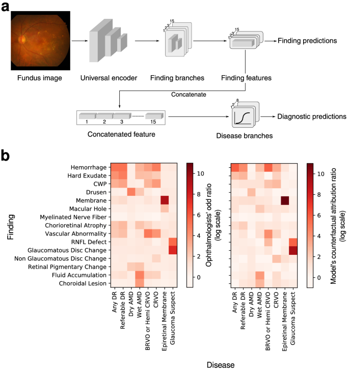
(a) Overall architecture of the deep learning-based model. (b) Relationships between ophthalmolgic findings and eye diseases computed by aggregate annotations of human experts and the model?EUR(TM)s counterfactual attribution ratio.
The finding-identification models and disease diagnosis models were trained and tested on data of 103,262 macula-centered fundus images from 47,764 patients (Supplementary Table 1). All models were evaluated with respect to its area under the receiver operating characteristic curve (AUROC), with its 95% confidence interval computed using the Clopper-Pearson method. Operating points were chosen to maximize the harmonic mean between sensitivity and specificity (i.e. F1-score) on the in-house validation data set except for BRVO/hemi-CRVO and CRVO whose operating points were set to have approximately 90% sensitivity because only a small number of positive cases were available.
Component #1: identification of fifteen abnormal findings
As shown in Table 1, the system identified findings in retinal fundus images with a mean AUROC of 0.980 across all 15 findings on a held-out, in-house test set. AUROCs ranged from a minimum of 0.972 for retinal pigmentary change to a maximum of 1.000 for myelinated nerve fiber layer with respect to the majority consensus of three ophthalmologists as reference. Sensitivities ranged from 92.5% for glaucomatous disc change to 100.0% for myelinated nerve fiber and specificity varied between 88.3% for retinal pigmentary change to 100.0% for myelinated nerve fiber (Supplementary Table 2, Supplementary Fig.? 1). This performance is comparable to human experts as reported in previous literature.12.
The models were then validated on 4 external datasets without additional tuning to identify findings included in each dataset: MESSIDOR17 (left( ) is the number of images with finding (k). We found that the average cosine distance between finding pairs started to increase beyond ?EUR~Block5a?EUR(TM) as in Supplementary Figs.? 4 and 5, signifying that feature maps at ?EUR~Block4a?EUR(TM) convey universal features informative of all findings whereas deeper layers learn discriminative features specific to each finding. We thus branched out after ?EUR~Block4a?EUR(TM). The encoder was then frozen to fine-tune finding branches until the validation AUROC saturated. Experimentally, the significant performance was not observed between architectures of different size that that we chose to append top layers of B0, the smallest network in the parameter size for each finding branch (Supplementary Table 5). Experimentally, freezing the encoder has minor effect in the test and validation AUROC on the in-house dataset (Supplementary Fig.? 6).
Target labels were assigned using the aforementioned Na??ve Bayes and the model was trained using the sum of BCE and guidance loss29. Training samples were randomly sampled non-uniformly in batches of size 6 such that the expected number of positive and negative samples in a batch are equal. The B7-B0 network was trained using Nesterov-SGD, with initial learning rate set to 0.001 until the 9th epoch reduced by a factor of 10 at epoch 10, until the validation AUROC decreased. Both linear projection matrices were trained for a maximum of 10 epochs with batch size 64 using the same Nesterov-SGD with L2-regularization coefficient 0.0005. Other training details such as augmentation and sampling ratio were identical to that used for training the B7-B0 network. The learning curves are illustrated in Supplementary Fig.? 7. In the experiment on predicting whether a fundus is normal, this final architecture did not show any degradation in AUROC compared to end-to-end models and other models with addition parameters (Supplementary Table 3).
Quantifying clinical relations between finding-disease pairs
To understand how our DL-based CAD system infers its diagnostic predictions, CAR was defined as a measure of how much a specific finding contributed to diagnosing a certain disease by comparing its prediction with what its prediction would have been in a hypothetical situation in which the finding under consideration is present or absent. Before defining CAR, we first define instance-dependent counterfactual attribution which can be computed for all finding-disease pairs (left( f,d right)) in a fundus image (x). First notice how the finding features (overlinez_f) can be decomposed as (overlinez_f = overlinez_ fracw_f + overlinez_f, bot w_f ) with a component (overlinez_w_f ) parallel to (w_f) and its orthogonal counterpart (overlinez_f, bot w_f ):
The odds (mathcalOleft( d;x right)) of disease (d) given a fundus image (x) is defined as the ratio between the model?EUR(TM)s prediction for disease (d) being present and absent:
Let the latent vector (overlinez_backslash f = left( sigma^ – 1 left( epsilon right) – b_f right)fracw_f w_f right + overlinez_f, bot w_f ) be the hypothetical feature map had the feature corresponding to finding (f) not been present in the image. The instance-dependent counterfactual attribution of finding (f) in diagnosing disease (d) from a fundus image (x) is the odds after removing the diagnostic prediction?EUR(TM)s dependency on finding (f), hence its name counterfactual:
For a finding-disease pair (left( f,d right)) and finding prediction? (haty_f) on a fundus image (x), the instance-dependent counterfactual attribution ratio (I-CAR) (R_I – CAR left( f,d;x right)) is the ratio between the odds and the counterfactual attribution:
where (sigma^ – 1) is the inverse sigmoid function and (epsilon in left( 0, 1/100 right)) is a small positive number. If a user wishes to modify the attribution due to some finding prediction, the diagnostic prediction of diseases is modified accordingly by changing (haty_f) in (overlinez_f). This is useful when a user wants to reject model?EUR(TM)s finding prediction in case of false positives and false negatives.
The two quantities described above establish the key intuition behind our main notion of CAR used to understand the decision-making process behind the DL-based CAD system. Replacing the prediction (haty_f) in I-CAR with a high confidence of (1 – epsilon) is the finding-disease CAR, comparing two hypothetical situations in which a finding is present surely and absent with high confidence:
The confidence level (epsilon) was chosen to be the 5-percentile ordered statistic of prediction values on benign cases in the in-house validation dataset.
Given a finding-disease pair, an attribution activation map that quantifies the influence of each finding (f) in diagnosing disease (d) can be visualized by modifying the class activation map13 as
Computation of odds ratios for human experts
Odds ratio of human experts were computed as following. Let (S) and (I) denote the set of annotator and image indices. Every image (x_i) indexed by (i) is associated with a finding (f_i^s) and disease (d_i^s) label indicating its presence of finding/diagnosis assigned by reader (s in S). All annotations were accumulated into a single (2 times 2) matrix (N) as
where (wedge) is the Boolean And operation and (1left cdot right\) is the indicator function. The odds ratio was then computed as
External datasets
The proposed models were tested on 9 external datasets with their summary statistics described in Supplementary Table 6. Two datasets, MESSIDOR and STARE, contain both findings and disease annotations, whereas 2?EUR”e-ophtha and IDRiD-segmentation?EUR”contain only finding annotations and 5 contain disease annotations: Kaggle-APTOS (2019), IDRiD-classification, REFUGE (training), REFUGE (val, test), and ADAM.
MESSIDOR consists of 1200 macula-centered images taken by TOPCON TRC NW6 digital fundus camera [TOPCON, Tokyo, Japan] with a 45-degree field of view. The dataset provides DR grades in a scale of 4, from 0 to 3, which does not align with the 5-scale grading in ICDRDSS. Three retinal specialists (SJP, JYS, HDK) who participated in annotating the in-house data independently assessed the images in the dataset regarding 15 findings and 8 diseases and adjusted the annotations to be compatible with the ICDRDSS grading. Images considered ungradable by any of the 3 specialists were excluded from our study.
All the other 8 external datasets are public datasets available online. Assessments provided with the datasets were used as-is when the decisions were binary (present/absent or positive/negative). Annotations in ICDRDSS scales in Kaggle-APTOS and IDRiD?EUR”classification datasets were converted to binary annotations for DR for grades (ge 1) and referable DR for grades (ge 2). Binary labels in the ADAM dataset indicate the presence of AMD without subcategorizing as dry or wet AMD, and the two subcategories were grouped into a single AMD class with annotations assigned positive/present if either dry or wet AMD was present and absent otherwise. The higher of predictions on dry and wet AMD were used to evaluate the model. The laterality of an image was derived by the center of the optic disc using a segmentation network for optic disc37, e.g. right eye if the disc center is on the right side.
Comparison with readers performance
To compare with human readers?EUR(TM) performance, 150 fundus images corresponding to 150 distinct subjects were sampled at the health screening center and ophthalmology outpatient clinic at SNUBH from July 1st, 2016 to June 30th, 2018. The images were captured with various fundus cameras including VX-10??, nonmyd 7, nonmyd WX [Kowa Optimed, Tokyo, Japan] with varying resolutions of (2144, 1424), (2992, 2000), (2464, 1632), (4288, 2848), and the data were annotated in disease names. Average age was 59.4 with standard deviation of 11.9 and there were 74 females (49.7%). The sampled data included cases of 25 DR (14 referable DR), 27 AMD (17 dry AMD, 10 wet AMD), 20 RVO (10 CRVO, 10 BRVO/hemi-CRVO), 13 glaucoma suspect, and 18 epiretinal membrane. We measured the performance of 4 physicians, and compared the performance with that of the DL algorithm. This dataset is denoted as ?EUR~Reader Study?EUR(TM) and the operating point of each reader is shown in Fig.? 2.
Data availability
Although public datasets are available at their respective repositories, SNUBH dataset is only available upon reasonable request to corresponding authors with the permission of the institution due to patient information protection law in Republic of Korea.
Code availability
We used the scikit-learn (https://scikit-learn.org) and statsmodels (https://www.statsmodels.org) packages to conduct the statistical tests in computing the AUROCs using the exact Clopper-Pearson method and confidence intervals. The machine-learning models were developed by using standard model libraries and scripts in TensorFlow and Keras. Custom code was specific to our computing infrastructure and mainly used for data input/output and parallelization across computing nodes. Proprietary codes for training and the deployment of the CAD system are not publicly available but some boilerplate code may be available for research purposes from the corresponding author upon reasonable request.
Abbreviations
- AMD:
-
Age-related macular degeneration
- AUROC:
-
Area under the receiver operating characteristic curve
- BRVO:
-
Branch retinal vein occlusion
- CAR:
-
Counterfactual attribution ratio
- CRVO:
-
Central retinal vein occlusion
- CWP:
-
Cotton wool patch
- DL:
-
Deep learning
- DNN:
-
Deep neural network
- DR:
-
Diabetic retinopathy
- ICDRDSS:
-
International Clinical Diabetic Retinopathy Disease Severity Scale
- IDRiD:
-
Indian Diabetic Retinopathy image Dataset
- REFUGE:
-
REtinal FUndus Glaucoma challengE
- RNFL:
-
Retinal nerve fiber layer
- RVO:
-
Retinal vein occlusion
- SNUBH:
-
Seoul National University Bundang Hospital
- t-SNE:
-
t-distributed stochastic neighbor embedding
References
-
Early Treatment Diabetic Retinopathy Study Research Group. Grading diabetic retinopathy from stereoscopic color fundus photographs?EUR”an extension of the modified Airlie house classification ETDRS report number 10. Ophthalmology 98, 786?EUR”806 (1991).
-
Detry-Morel, M. et al. Screening for glaucoma in a general population with the non-mydriatic fundus camera and the frequency doubling perimeter. Eur. J. Ophthalmol. 14, 387?EUR”393 (2004).
-
Chew, E. Y. et al. The age-related eye disease study 2 (AREDS2): Study design and baseline characteristics (AREDS2 report number 1). Ophthalmology 119, 2282?EUR”2289 (2012).
-
The Eye Disease Case-control Study Group. Risk factors for branch retinal vein occlusion. Am. J. Ophthalmol. 116, 286?EUR”296 (1993).
-
LeCun, Y., Bengio, Y. & Hinton, G. Deep learning. Nature 521, 436?EUR”444. https://doi.org/10.1038/nature14539 (2015).
-
Gulshan, V. et al. Development and validation of a deep learning algorithm for detection of diabetic retinopathy in retinal fundus photographs. JAMA 316, 2402?EUR”2410. https://doi.org/10.1001/jama.2016.17216 (2016).
-
Ting, D. S. W. et al. Development and validation of a deep learning system for diabetic retinopathy and related eye diseases using retinal images from multiethnic populations with diabetes. JAMA 318, 2211?EUR”2223. https://doi.org/10.1001/jama.2017.18152 (2017).
-
Li, Z. et al. Efficacy of a deep learning system for detecting glaucomatous optic neuropathy based on color fundus photographs. Ophthalmology 125(8), 1199?EUR”1206 (2018).
-
Asaoka, R., Murata, H., Iwase, A. & Araie, M. Detecting preperimetric glaucoma with standard automated perimetry using a deep learning classifier. Ophthalmology 123, 1974?EUR”1980. https://doi.org/10.1016/j.ophtha.2016.05.029 (2016).
-
Burlina, P. M. et al. Automated grading of age-related macular degeneration from color fundus images using deep convolutional neural networks. JAMA Ophthalmol. 135, 1170?EUR”1176 (2017).
-
Peng, Y. et al. DeepSeeNet: A deep learning model for automated classification of patient-based age-related macular degeneration severity from color fundus photographs. Ophthalmology 126, 565?EUR”575. https://doi.org/10.1016/j.ophtha.2018.11.015 (2019).
-
Son, J. et al. Development and validation of deep learning models for screening multiple abnormal findings in retinal fundus images. Ophthalmology https://doi.org/10.1016/j.ophtha.2019.05.029 (2019).
-
Zhou, B., Khosla, A., Lapedriza, A., Oliva, A. & Torralba, A. in Proceedings of the IEEE Conference on Computer Vision and Pattern Recognition. pp. 2921?EUR”2929.
-
Selvaraju, R. R. et al. in Proceedings of the IEEE International Conference on Computer Vision. pp. 618?EUR”626.
-
Sundararajan, M., Taly, A. & Yan, Q. in Proceedings of the 34th International Conference on Machine Learning, Vol. 70. 3319?EUR”3328 (JMLR. org).
-
Park, S. J. et al. A novel fundus image reading tool for efficient generation of a multi-dimensional categorical image database for machine learning algorithm training. J Korean Med Sci 33 (2018).
-
Decenci??re, E. et al. Feedback on a publicly distributed image database: The Messidor database. Image Anal. Stereol. 33, 231?EUR”234 (2014).
-
Decenciere, E. et al. TeleOphta: Machine learning and image processing methods for teleophthalmology. Irbm 34, 196?EUR”203 (2013).
-
Prasanna Porwal, S. P. R. K., Manesh Kokare, Girish Deshmukh, Vivek Sahasrabuddhe and Fabrice Meriaudeau. (IEEE Dataport, 2018).
-
Adam, H. STARE database, http://www.ces.clemson.edu/~ahoover/stare (2004).
-
Orlando, J. I. et al. REFUGE challenge: A unified framework for evaluating automated methods for glaucoma assessment from fundus photographs. Med. Image Anal. 59, 101570. https://doi.org/10.1016/j.media.2019.101570 (2019).
-
Fu, H., Li, F., Orlando, J. I., Bogunovi??, H., Sun, X., Liao, J., Xu, Y., Zhang, S., Zhang, X. ADAM: Automatic Detection challenge on Age-related Macular degeneration (IEEE DataPort, 2020).
-
Montavon, G., Lapuschkin, S., Binder, A., Samek, W. & M? 1/4 ller, K.-R. Explaining nonlinear classification decisions with deep Taylor decomposition. Patt. Recogn. 65, 211?EUR”222 (2017).
-
Lundberg, S. & Lee, S.-I. A unified approach to interpreting model predictions. arXiv preprint http://arxiv.org/abs/1705.07874 (2017).
-
Singh, A., Sengupta, S. & Lakshminarayanan, V. Explainable deep learning models in medical image analysis. J. Imag. 6, 52 (2020).
-
Qayyum, A., Anwar, S. M., Awais, M. & Majid, M. Medical image retrieval using deep convolutional neural network. Neurocomputing 266, 8?EUR”20 (2017).
-
Lee, H. et al. An explainable deep-learning algorithm for the detection of acute intracranial haemorrhage from small datasets. Nat. Biomed. Eng. 3, 173?EUR”182 (2019).
-
Kim, B. et al. in International Conference on Machine Learning. 2668?EUR”2677 (PMLR).
-
Son, J., Bae, W., Kim, S., Park, S. J. & Jung, K-H. Computational Pathology and Ophthalmic Medical Image Analysis 176?EUR”184 (Springer, 2018).
-
Son, J., Kim, S., Park, S. J. & Jung, K-H. in Intravascular Imaging and Computer Assisted Stenting and Large-Scale Annotation of Biomedical Data and Expert Label Synthesis: 7th Joint International Workshop, CVII-STENT 2018 and Third International Workshop, LABELS 2018, Held in Conjunction with MICCAI 2018, Granada, Spain, September 16, 2018, Proceedings 3. 95?EUR”104 (Springer).
-
Collins, M. The naive bayes model, maximum-likelihood estimation, and the em algorithm. Lecture Notes (2012).
-
Tan, M. & Le, Q. V. EfficientNet: Rethinking Model Scaling for Convolutional Neural Networks. arXiv preprint http://arxiv.org/abs/1905.11946 (2019).
-
Kendall, A., Gal, Y. & Cipolla, R. in Proceedings of the IEEE Conference on Computer Vision and Pattern Recognition. pp. 7482?EUR”7491.
-
Teichmann, M., Weber, M., Zoellner, M., Cipolla, R. & Urtasun, R. in 2018 IEEE Intelligent Vehicles Symposium (IV). pp. 1013?EUR”1020 (IEEE).
-
Liao, Y., Kodagoda, S., Wang, Y., Shi, L. & Liu, Y. in 2016 IEEE international conference on robotics and automation (ICRA). pp. 2318?EUR”2325 (IEEE).
-
Maaten, L. V. D. & Hinton, G. Visualizing data using t-SNE. J. Mach. Learn. Res. 9, 2579?EUR”2605 (2008).
-
Son, J., Park, S. J. & Jung, K. H. Towards accurate segmentation of retinal vessels and the optic disc in fundoscopic images with generative adversarial networks. J. Digit. Imaging 32, 499?EUR”512. https://doi.org/10.1007/s10278-018-0126-3 (2019).
Funding
This study was supported by the Research Grant for Intelligence Information Service Expansion Project, which is funded by National IT Industry Promotion Agency (NIPA-C0202-17-1045), the Basic Science Research Program through the National Research Foundation of Korea (NRF) (NRF-2021R1C1C1014138), and Korea Environment Industry & Technology Institute (KEITI) through the Core Technology Development Project for Environmental Diseases Prevention and Management, funded by Korea Ministry of Environment (MOE) (grant number: 2022003310001). The sponsors or funding organizations had no role in the design or conduct of this research.
Author information
Authors and Affiliations
Contributions
J.S., J.Y.S., K-H.J., S.J.P. conceptualized the work. J.S. developed the model. K-H.J. advised the modeling technique. J.S., J.Y.S., K-H.J., S.J.P. wrote the manuscript. S.T.K revised method part. J.P., G.K. created the figures. J.Y.S, H.D.K., K.H.P., S.J.P. provided clinical expertise. K-H.J. and S.J.P. supervised the work.
Corresponding authors
Ethics declarations
Competing interests
J.S, S.T.K., J.P., G.K. are employee of VUNO Inc.. K-H.J. and S.J.P are shareholders of VUNO Inc., Seoul, South Korea. J.Y.S, H.D.K., K.H.P. declares they have no competing interests.
Additional information
Publisher’s note
Springer Nature remains neutral with regard to jurisdictional claims in published maps and institutional affiliations.
Supplementary Information
Rights and permissions
Open Access This article is licensed under a Creative Commons Attribution 4.0 International License, which permits use, sharing, adaptation, distribution and reproduction in any medium or format, as long as you give appropriate credit to the original author(s) and the source, provide a link to the Creative Commons licence, and indicate if changes were made. The images or other third party material in this article are included in the article’s Creative Commons licence, unless indicated otherwise in a credit line to the material. If material is not included in the article’s Creative Commons licence and your intended use is not permitted by statutory regulation or exceeds the permitted use, you will need to obtain permission directly from the copyright holder. To view a copy of this licence, visit http://creativecommons.org/licenses/by/4.0/.
About this article
Cite this article
Son, J., Shin, J.Y., Kong, S.T. et al. An interpretable and interactive deep learning algorithm for a clinically applicable retinal fundus diagnosis system by modelling finding-disease relationship.
Sci Rep 13, 5934 (2023). https://doi.org/10.1038/s41598-023-32518-3
-
Received:
-
Accepted:
-
Published:
-
DOI: https://doi.org/10.1038/s41598-023-32518-3
Comments
By submitting a comment you agree to abide by our Terms and Community Guidelines. If you find something abusive or that does not comply with our terms or guidelines please flag it as inappropriate.
right)) for all 15 findings, e-ophtha18 (left( n = 434 right)) for hemorrhage and hard exudate, IDRiD-segmentation19 (left( n = 143 right)) for hemorrhage, hard exudate, and CWP, as well as STARE20 (left( n = 397 right)) for the presence of myelinated nerve fiber. On the MESSIDOR dataset, which consists of external images internally annotated by three retinal specialists (PSJ, SJY, KHD), the model achieved an average AUROC of 0.915 with a minimum of 0.804 for retinal pigmentary change to a maximum of 1.0 for macular hole and myelinated nerve fiber layer. Sensitivity on the MESSIDOR dataset was rather compromised ranging from 42.5% for drusen to 100.0% for myelinated nerve fiber and macular hole while specificity was comparable to that of the in-house test set ranging from 88.3% for hard exudate to 100.0% for myelinated nerve fiber. On external datasets from multiple sources, the model attained AUROCs ranging from 0.964 (e-ophtha, hard exudate) to 1.000 (IDRiD, hard exudate). Sensitivity was comparable to that of the in-house test set with a minimum of 85.1% (e-ophtha, hemorrhage), but specificity dropped in certain datasets down to a minimum of 65.7% (e-ophtha, hard exudate).
Component #2: diagnosis of eight major eye diseases
The diagnostic performance of the disease models trained on top of the finding models reached a mean AUROC of 0.992 across all 8 diseases in the in-house, held-out test set, ranging from 0.979 for glaucoma suspect to 0.999 for referable DR (Table 1 and Fig.? 2). This performance carried on to the MESSIDOR and all 6 external datasets: MESSIDOR ((n = 1189)) with an average AUROC of 0.959 ranging from 0.938 for dry AMD to 0.983 for referable DR, Kaggle APTOS-2019 challenge (left( n = 3662 right)) with 0.986 AUROC averaged over DR and referable DR, IDRiD-classification19 (left( n = 3662 right)) with average AUROC of 0.968 for the same diseases, 0.951 and 0.967 for glaucoma suspect on REFUGE21 (training) (left( n = 400 right)) and REFUGE21 (val, test) (left( n = 800 right)) respectively, 0.943 for dry and wet AMD on ADAM22 (left( n = 400 right)), and 0.964 averaged across CRVO, BRVO/hemi-CRVO, and epiretinal membrane on STARE (left( n = 397 right)). The disease diagnosis models?EUR(TM) receiver operating characteristic curves in Fig.? 2 are comparable to that of four physicians?EUR(TM) operating points, demonstrating their practicality as a comprehensive CAD system. However, as observed for the finding models, diagnostic models exhibited either exclusively high sensitivity or specificity on some datasets with a minimum sensitivity of 77.8% (MESSIDOR, glaucoma suspect) and minimum specificity of 69.0% (IDRiD, DR).
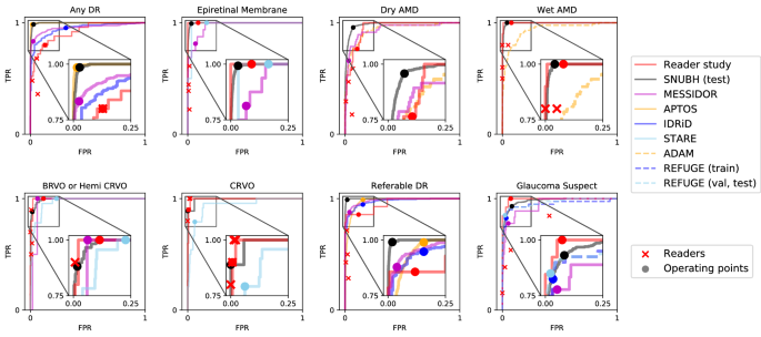
Receiver operating characteristic curves for diseases. Gray boxes are amplified to present the profile of the curves in a practical range. Operating points of the models are marked with circles and performance of human readers are plotted with cross marks. Receiver operating characteristic curves for ADAM dataset is identical for dry AMD and wet AMD.
Quantification of clinical relations between findings and diseases
The unique finding-disease network architecture permits the use of a newly defined notion of CAR of each finding-disease pair as detailed in the ?EURoeMethods?EUR? Section. CAR quantifies the extent to which the model?EUR(TM)s diagnostic prediction attributes to a finding by comparing the disease diagnosis model?EUR(TM)s predictions under two hypothetical situations in which the finding of interest had been present or absent with absolute confidence. This notion is directly comparable to the odds ratio calculated for human experts, and can be interpreted as a measure of the clinical relation between finding-disease pairs. The similarity of CARs for all finding-disease pairs from our CAD system and odds ratio collectively estimated over 57 board-certified ophthalmologists on the in-house test dataset demonstrates how both entities generate similar diagnostic opinions (Fig.? 1b). The network associated diseases with findings as following: DR and referable DR with hemorrhage and hard exudate that are key clinical findings used to diagnose the severity of DR; dry AMD with drusen; wet AMD with fluid accumulation, choroidal lesion, and hemorrhage; RVO with hemorrhage, CWP, vascular abnormality; epiretinal membrane with membrane but not macular hole, although epiretinal membrane and macular hole frequently occur together as shown in the human?EUR(TM)s odds ratio; glaucoma suspect with glaucomatous disc change and RNFL defect. The agreement between the model?EUR(TM)s CAR values and human experts?EUR(TM) odds ratio reveals the similar attribution of identified findings in diagnostic predictions as in medical practice. Figure? 3 illustrates how our CAD system can visualize the model?EUR(TM)s attribution ratio between finding-disease pairs.
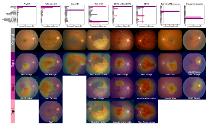
Use cases of counterfactual attribution ratio in diagnostic fundus examination. Lesions of top 3 findings above a threshold (natural constant e) are shown (attribution activation map).
To compensate for the inevitable imperfection of deep neural networks (DNNs), a CAD system should ideally be interactive when readers disagree with the model?EUR(TM)s finding identification or diagnostic prediction partially or entirely. Figure? 4 shows how a reader can interact with this CAD system to reduce or increase the influence of a certain finding on the model?EUR(TM)s diagnostic prediction, by modifying the finding?EUR(TM)s prediction score between values of 0 and 1. For example, if the reader thinks the model missed the diagnosis of glaucoma suspect due to underestimation of the presence of glaucomatous disc change, the reader may simply modify the attribution of glaucomatous disc change to 1 and obtain its corresponding diagnostic prediction of glaucoma suspect. This ?EUR~physician-in-the-loop?EUR(TM) procedure does not require an additional inference step and the re-evaluation incurs negligible computation. This is especially useful when the mis-identification is due to sensor error such as a stain on the camera?EUR(TM)s lens identified as hemorrhage or CWP15. The interactive diagnosis enabled by the use of the CAR framework ultimately makes the models?EUR(TM) diagnostic predictions readily adaptable to noise or ambiguity pervasive in practical clinical settings.
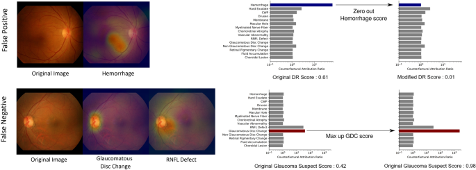
Interactive diagnosis using counterfactual attribution ratio and the attribution maps of relevant findings. (top) A false-positive diagnosis of diabetic retinopathy can be corrected by suppressing the overestimated attribution of hemorrhage. (bottom) A false-negative diagnosis of glaucoma can be corrected by increasing the underestimated attribution of glaucomatous disc change.
Hemorrhage feature maps for various different diagnoses
During the annotation process, various types of one finding were grouped into a broader super-class to enhance simplicity in the model and also for efficiency in obtaining large-scale labeled datasets12,16. For example, various sub-types of hemorrhage such as flame-shaped hemorrhage, dot hemorrhage, splinter hemorrhage, blot hemorrhage, subretinal hemorrhage, preretinal hemorrhage, vitreous hemorrhage were all classified as one super-class hemorrhage; however, a fine-grained classification of the findings critically effects diagnostic conclusions. A model trained to classify the super-class may be unable to discriminate precise patterns corresponding to different sub-findings and consequently yield incorrect diagnostic predictions. Figure? 5 visualizes the latent spaces of different sub-features by projecting features extracted from the in-house test set using t-Distributed Stochastic Neighbor Embedding (t-SNE). Feature maps for hemorrhage were extracted for positive cases of DR, RVO, and wet AMD, where positive cases were defined as an agreement of more than two independent annotators. Three clusters in large represent each disease showing different patterns of hemorrhage. Samples of DR show dot hemorrhage and blot hemorrhage in localized areas, and RVO cases include flame-shaped hemorrhage in a broad area while intraretinal and subretinal hemorrhage of all shapes and sizes are possible in cases of wet AMD. Several outliers for wet AMD on the left side of the t-SNE plot comprise small amounts of bleeding, resembling blot hemorrhage. From this, it is evident that although the model does not have access to fine-grained specifications of types of sub-findings, different sub-categories of hemorrhage and their corresponding patterns are well-preserved.
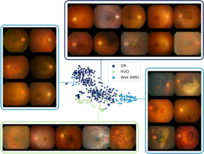
t-Distributed Stochastic Neighbor Embedding plots of hemorrhage feature maps for positive cases of diseases that involve hemorrhage in diagnostic decisions.
